04 ML regression 03

Value of the Information & Strength of the Argument

The informational value lies in a complete, self-contained walkthrough of the closed-form solution to simple linear regression. The instructor does not merely state the formula beta1 = Cov(X,Y)/Var(X); he builds it from the residual-sum-of-squares objective, shows the two normal equations obtained by partial differentiation, and explicitly motivates the algebraic trick of adding and subtracting Xbar terms by demonstrating that the added quantity equals zero and therefore leaves the expression unchanged while making it factorisable. This is a genuinely useful pedagogical move, because it explains why the covariance/variance form appears in libraries and packages rather than presenting it as a black box. The worked numerical example is well chosen: with only five samples the student can verify each intermediate quantity by hand, and the instructor checks the fitted line against the training points (predicting 1.2 for x = 1 where 1 was expected, 2 for x = 2 where 3 was expected) to make the notion of residual concrete. The argumentation is sound and linear, moving from objective to derivation to implementation to generalisation. Its weaknesses are that the reasoning is entirely deductive and internal — no data, no validation, no discussion of assumptions (linearity, homoscedasticity, independence of errors), no mention of when OLS fails or of alternatives such as regularisation. The generalisation to multivariate regression is announced and set up (the x0 = 1 augmentation, the design matrix X, the compact Y_hat = X*theta form) but the derivation itself is postponed, so the session ends on an incomplete argument. The Python code is presented as a direct transcription of the algebra, which is a strength for learners, but the instructor explicitly withholds the plotting code and warns against copying, which limits reproducibility of the full exercise from the video alone.

Scientific Rigor, Source Quality, Title Accuracy

Rigueur scientifique : the mathematics is standard textbook material and is handled correctly. The derivation of the normal equations, the substitution of beta0 into the beta1 equation, and the covariance/variance reduction are all valid, and the numerical result for the five-point example is consistent with the stated data. The instructor is careful to flag the zero-sum trick as not changing the equation, which is exactly the kind of justification that distinguishes a rigorous derivation from a memorised one. The main scientific gaps are the absence of any statement of the OLS assumptions, of the conditions under which the closed-form solution exists (invertibility of X’X), and of any error or uncertainty analysis on the fitted coefficients. Qualité des sources : no sources are cited. The video description is empty, there are no chapters, no references to textbooks, papers or documentation, and no links of any kind. The content therefore rests entirely on the instructor’s own exposition, which happens to be correct but is unverifiable against any named authority within the video itself. Adéquation titre/contenu : the title ‘04 ML regression 03’ is a bare course-index label; it is consistent with the content (third regression session of a machine-learning course) but conveys essentially nothing to a viewer, and the final minutes drift into an unrelated syllabus discussion.

7/10

The mathematical content is standard, correct and internally consistent: the OLS derivation from the squared-error minimisation to the closed-form beta1 = Cov(X,Y)/Var(X) is carried out step by step and verified on a small worked example (five points, beta0 = 0.4, beta1 = 0.8). The Python implementation mirrors the algebra exactly. No external claims, statistics or empirical results are asserted, so there is little room for factual error; the score is limited mainly by the absence of any cited reference, textbook or dataset, and by the informal, lecture-hall delivery with repeated interruptions about screen visibility.

Markers derived by PSI from the transcript: the creator did not define chapters.

• 00:00Framing of regression as estimating Y = f(X) with a linear f, and definition of the squared-error / RMSE objective summed over all samples.
• 02:30Distinction between univariate and multivariate regression: one feature gives a line, several give a plane or hyperplane.
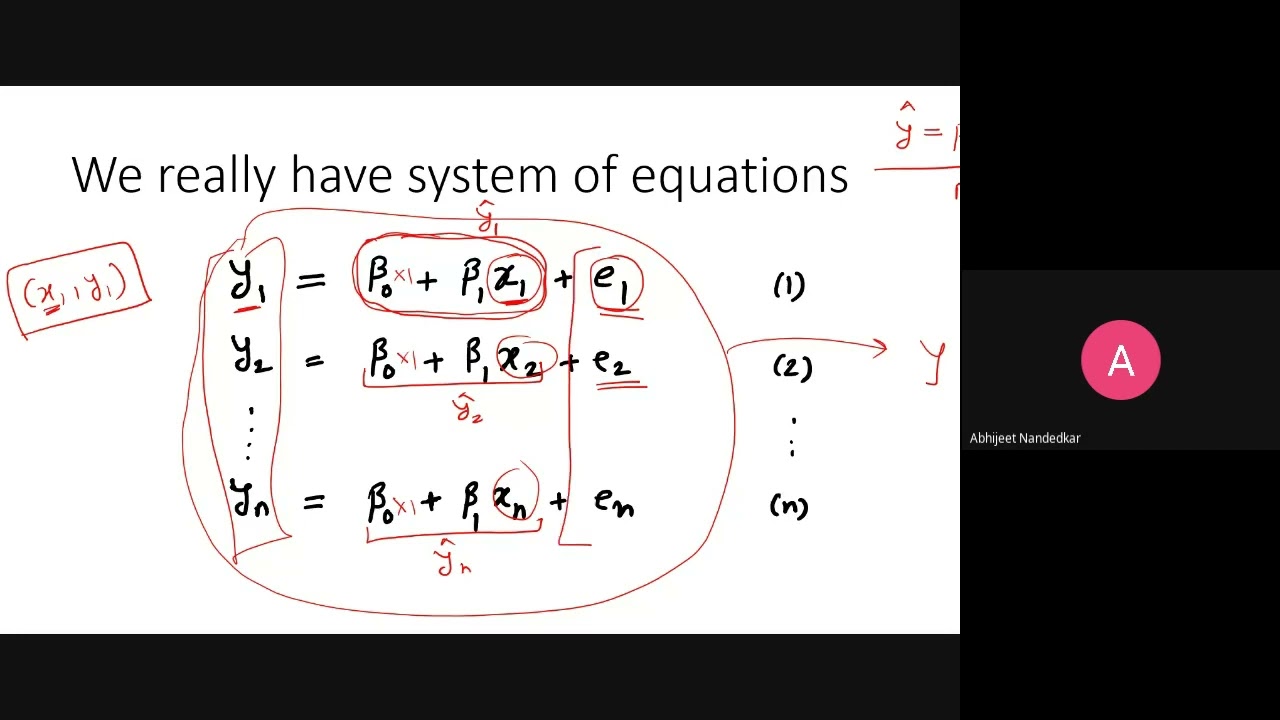
• 05:00Setup of the model y_i = beta0 + beta1*x_i + e_i and statement that the betas are the unknowns to be fitted.
• 08:00Matrix representation of the system: Y = A*beta + e, with the column of ones augmented into A.
• 10:00Minimisation of the squared norm of the error vector by differentiation with respect to beta0, giving beta0 = Ybar - beta1*Xbar.
• 13:00Differentiation with respect to beta1, substitution of beta0, and simplification of the resulting expression.
• 16:00The zero-sum algebraic trick: adding and subtracting Xbar terms to factorise numerator and denominator.
• 19:00Identification of the final result: beta1 = Cov(X,Y)/Var(X), with definitions of covariance and variance.
• 21:00Worked example with five samples and the Python implementation using mean, covariance and variance functions.
• 26:00Numerical result beta0 = 0.4, beta1 = 0.8, and verification of the fitted line against the training points.
• 30:00Generalisation to d features: coefficients renamed theta, artificial x0 = 1 column, compact form Y_hat = X*theta.
• 39:00Transition to an unrelated administrative discussion about a DSP practical being added to the syllabus.