lect19 Naïve Bayes Classifier
Keywords
Summary
232 words
Critical Evaluation
Value of the Information & Strength of the Argument
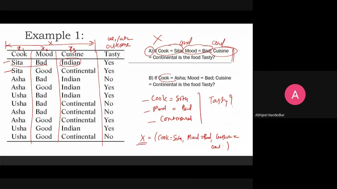
The informational value lies in the worked examples rather than in any conceptual novelty. The instructor’s central pedagogical move is well chosen: by selecting queries that are absent from the training table, he makes the motivation for Naïve Bayes concrete and immediate. A reader sees exactly why a pure lookup or a full joint-frequency estimate fails, and how the independence assumption rescues the computation. The step-by-step arithmetic — counting six ‘yes’ out of ten, then two ‘Sita’ among those six, then two ‘bad mood’ among those six, then two ‘Continental’ among those six — is transparent and can be followed and reproduced by hand, which is a genuine strength for a learner. The treatment of the zero-frequency problem is also practically valuable: the instructor explicitly warns against leaving a zero in the product, since it annihilates the entire likelihood, and recommends a small replacement value. He further demonstrates a useful trick for obtaining exact posteriors without computing P(X) directly, by using the fact that the two class posteriors sum to one and solving for the normalising constant. The argumentation is, however, entirely operational. The independence assumption is presented as a computational convenience (’the way out is that we assume all the variables are independent’) with no discussion of when it is defensible, what happens when features are strongly correlated, or why the classifier can still work well in practice despite a violated assumption. The choice of smoothing constant is justified only by intuition (‘don’t put big values like 0.1 or 0.2’), with no mention of additive or Laplace smoothing, no formula, and no discussion of how the constant interacts with sample size. The distinction between the maximum a posteriori decision rule and calibrated probability estimates is touched on implicitly but never stated. The lecture is also delivered informally, with audible self-corrections and a partially incoherent opening, which slightly reduces its clarity as a standalone resource.
Scientific Rigor, Source Quality, Title Accuracy
On scientific rigour, the mathematical content presented is correct: the factorisation of the likelihood under conditional independence, the use of class priors, the comparison of unnormalised posteriors for classification, and the recovery of normalised posteriors via the sum-to-one constraint are all standard and correctly executed. The arithmetic checks out in both examples. The main rigour gap is the absence of any formal statement of the model, any notation defined cleanly, and any reference to the underlying literature. The zero-frequency remedy is described only qualitatively, without naming additive smoothing or giving the estimator, which is a notable omission for a topic where that detail is the standard textbook treatment. On sources, the video cites none: there is no bibliography, no paper, no textbook, no dataset provenance, and the description contains no links at all. The two datasets appear to be invented for the exercise, which is acceptable for a tutorial but means nothing can be independently traced or verified. There is therefore no source quality to assess — the material stands or falls on its internal consistency alone. On title/content adequacy, the title ’lect19 Naïve Bayes Classifier’ is a precise and honest description of the content; there is no gap between what is promised and what is delivered. No comments were provided for analysis.
543 words
Title / Content Match
The title matches the content exactly: the video is a worked lecture on the Naïve Bayes classifier, applied to two tabular toy datasets. No mismatch between title and content.
Quality & Reliability
6/10
The lecture is technically sound on the core mechanics of Naïve Bayes: the conditional independence assumption, the likelihood/prior decomposition, the zero-frequency problem and Laplace-style smoothing, and the normalisation via the marginal P(X). The arithmetic is internally consistent and reproducible from the tables given. However, no sources, references or literature are cited, the smoothing constant is introduced as an arbitrary 'small number' without naming Laplace/additive smoothing or justifying the choice, and the treatment of the independence assumption is purely operational — its statistical cost (biased posteriors, correlated features) is never discussed. The presentation is informal and partly improvised, with several self-corrections and a garbled opening sentence, which limits its value as a reference document.
Key Moments
Markers derived by PSI from the transcript: the creator did not define chapters.
- Introduction of the first dataset: features cook, mood and cuisine, with a binary outcome (food tasty or not) over ten samples.
- Statement of the query whose feature combination is absent from the table, motivating the need for Naïve Bayes.
- Introduction of the conditional independence assumption between the three input variables.
- Computation of the class prior: six 'yes' out of ten samples.
- First likelihood term: P(cook = Sita | tasty = yes) = 2/6.
- Second likelihood term: P(mood = bad | tasty = yes) = 2/6.
- Third likelihood term: P(cuisine = Continental | tasty = yes) = 2/6.
- Assembly of the Naïve Bayes equation and computation of the unnormalised posterior for the 'yes' class.
- Treatment of the zero-frequency problem: replacing a zero probability with a small constant, with a warning against large values.
- Comparison of the two posteriors and decision rule; recovery of exact probabilities by solving for the normalising constant P(X).
- Second worked example on vehicle data: colour, type and origin as features, 'stolen' as the outcome.
- Final comparison of posteriors for the vehicle example and conclusion that the car is not stolen.
Contribution & Novelties
The video offers no original research contribution; it is a pedagogical walkthrough of a classical algorithm. Its value is didactic: the deliberate choice of queries absent from the training table makes the motivation for the independence assumption vivid, and the two fully worked examples — one on food, one on vehicles — give a learner a complete, hand-checkable template for applying Naïve Bayes to categorical tabular data. The demonstration that exact posterior probabilities can be recovered without explicitly computing P(X), by using the sum-to-one constraint, is a practical trick that is often glossed over in introductory treatments. The main limitation is that the method is presented purely as a computational device, with no discussion of the statistical consequences of the independence assumption or of the standard smoothing estimator.
Pour aller plus loin :
- Naive Bayes classifier — The standard reference article covering the model, the conditional independence assumption, and the variants (Bernoulli, multinomial, Gaussian).
- Additive smoothing — Covers the Laplace and Lidstone estimators that formalise the ‘small number’ replacement used in the video for zero-frequency cases.
- Bayes’ theorem — The foundational result underlying the posterior computation performed throughout the lecture.
- Maximum a posteriori estimation — Explains the decision rule implicitly used when comparing the two unnormalised posteriors.
- Tom M. Mitchell, Machine Learning, McGraw-Hill, 1997, chapter 6 — The classical textbook treatment of Naïve Bayes and its application to text classification.
230 words
Radar Profile
The profile is that of a low-to-moderate introductory tutorial: information quantity and quality sit in the middle range because the two examples are complete and correctly worked, while the technical level is low, reflecting a first-exposure treatment with no formal notation or statistical depth. Overall reliability is moderate — the mathematics is correct and reproducible, but the absence of any cited source, formal estimator for smoothing, or discussion of the independence assumption's limits caps the score.